Note
Go to the end to download the full example code or to run this example in your browser via Binder.
Guide to PUNCH Data#
A notebook guide to working with PUNCH FITS files in Python
This Jupyter Notebook presents a comprehensive guide to the analysis and visualization of PUNCH FITS files using Python. The guide leverages a suite of Python libraries, including matplotlib for data visualization, numpy for numerical operations, astropy for FITS file handling and WCS manipulation, sunpy for solar data analysis, and ndcube for multi-dimensional data handling. The notebook serves as a robust resource for researchers and scientists, providing them with the tools and knowledge to effectively manipulate and interpret PUNCH FITS files. The guide’s step-by-step approach, coupled with code snippets and detailed explanations, ensures a user-friendly experience, promoting the accessibility of PUNCH data for a wider scientific community.
To install these dependencies, use pip install -r requirements.txt in your terminal.
Load libraries
from copy import deepcopy

import astropy.units as u
import matplotlib.pyplot as plt
import numpy as np
from astropy.io import fits
from astropy.wcs import WCS
from matplotlib.colors import LogNorm
from ndcube import NDCube
from sunpy.map import Map

from punchbowl.data.sample import PUNCH_CAM, PUNCH_PAM
from punchbowl.data.visualize import plot_punch
Data loading#
We first specify the file we wish to load. For this notebook, let’s use the included L3 PAM file. Then, we’ll load it two different ways:
With astropy.io
With SunPy Maps
The data are RICE compressed, so we’ll have to look in the second at index 1 (since we’re zero-indexed) HDU for the main data frame. There is also an uncertainty layer in the last HDU that we’ll explore later.
with fits.open(PUNCH_PAM) as hdul:
    data = hdul[1].data
    header = hdul[1].header
    uncertainty = hdul[2].data
First, let’s look at the shape of the data. For this data product, total brightness and polarized brightness are stacked along the first dimension. The uncertainty array corresponds on a pixel-to-pixel basis with the data array.
print(data.shape, uncertainty.shape)
(2, 4096, 4096) (2, 4096, 4096)
We can look in the header for details about the data. A few things to note:
The header is divided into helpful sections such as “temporal information” and “instrument and spacecraft state.” This aids in navigating the information. These sections are consistent for other products (with the addition of more sections depending on the product).
There are two world coordinate systems (WCS), one for the helio system and one for a celestial right ascension and declination system. They match each other and can be used interchangeably depending on the type of analysis.
The first dimension iterates over total brightness and polarized brightness, in that order. This is indicated by the OBSLAYR1 and OBSLAYR2 keywords.
print(header)
SIMPLE = 'T ' / Conforms to FITS Standard BITPIX = -32 / Number of bits per pixel NAXIS = 3 / Number of axes NAXIS1 = 4096 / Length of the first axis NAXIS2 = 4096 / Length of the second axis NAXIS3 = 2 / Length of the third axis COMMENT ----- FITS Required ----------------------------------------------------EXTNAME = 'PRIMARY DATA ARRAY' / Name of this binary table extension LONGSTRN= 'OGIP 1.0' / The OGIP long string convention may be used COMMENT ----- Documentation, Contact, and Collection Metadata ------------------DOI = 'https://doi.org/TBD' / Data reference DOI PROJECT = 'PUNCH ' TITLE = 'PUNCH Level-3 Polarized Low Noise Mosaic' KEYVOCAB= 'Unified Astronomy Thesaurus Keywords' KEYWORDS= 'Solar Corona (1483), Solar K Corona (2042), Solar F Corona (1991), &'CONTINUE 'Solar Coronal Streamers (1486), Solar Coronal Plumes (2039), Solar &'CONTINUE 'Wind (1534), Fast Solar Wind (1872), Slow Solar Wind (1873), Solar &'CONTINUE 'Coronal Mass Ejection (310), Heliosphere (711), Polarimetry (1278)' LICENSE = 'Creative Commons Attribution 4.0 International | CC BY 4.0' DESCRPTN= 'PUNCH Level-3 data, Composite mosaic in output coordinates' DOC_URL = 'https://punch.spaceops.swri.org' COMMENT ----- File Type and Provenance -----------------------------------------FILENAME= '' / Name of file LEVEL = '3 ' / Product Level OBSTYPE = 'Polarized low noise mosaic' / Plain text observation TYPECODE= 'PA ' / Observation product type code OBSCODE = 'M ' / Observatory spacecraft code PIPEVRSN= '' / PUNCHPipe software version number FILE_RAW= '' / Raw telemetry filename ORIGIN = 'SwRI ' / Institution responsible for creating the file COMMENT ----- Temporal Information ---------------------------------------------TIMESYS = 'UTC ' / Principal time system DATE-BEG= '2024-06-20T00:00:00.000' / UTC time observation DATE-OBS= '2024-06-20T00:00:00.000' / UTC reference time DATE-AVG= '2024-06-20T00:16:00.000' / UTC reference time DATE-END= '2024-06-20T00:32:00.000' / UTC time of observation end DATE = '2024-06-20T12:32:00.000' / UTC file generation date and time COMMENT ----- Instrument and Spacecraft State ----------------------------------WAVELNTH= 530 / [nm] average peak response WAVEUNIT= 'nanometer' / Unit of observation measurement OBS-MODE= 'Polar_BpB' / Image Mode (Unpolarized, Polar_MZP, Polar_BpB) OBSLAYR1= 'Polar_B ' / Image Mode for first datacube layer OBSLAYR2= 'Polar_pB' / Image Mode for second datacube layer INSTRUME= 'WFI+NFI Mosaic' / Instrument name TELESCOP= 'PUNCH 1-2-3-4' / Satellite name OBSRVTRY= 'PUNCH ' / Observatory name OBJECT = 'Heliosphere white light' / Object observed COMMENT ----- World Coordinate System ------------------------------------------WCSAXES = 3 / Number of coordinate axes CRPIX1 = 2047.5 / Pixel coordinate of reference point CRPIX2 = 2047.5 / Pixel coordinate of reference point CRPIX3 = 0.0 / Pixel coordinate of reference point PC1_1 = 1.0 / Coordinate transformation matrix element PC1_2 = 0.0 / Coordinate transformation matrix element PC1_3 = 0.0 / Coordinate transformation matrix element PC2_1 = 0.0 / Coordinate transformation matrix element PC2_2 = 1.0 / Coordinate transformation matrix element PC2_3 = 0.0 / Coordinate transformation matrix element PC3_1 = 0.0 / Coordinate transformation matrix element PC3_2 = 0.0 / Coordinate transformation matrix element PC3_3 = 1.0 / Coordinate transformation matrix element CDELT1 = 0.0225 / [deg] Coordinate increment at reference point CDELT2 = 0.0225 / [deg] Coordinate increment at reference point CDELT3 = 1.0 / Coordinate increment at reference point CUNIT1 = 'deg ' / Units of coordinate increment and value CUNIT2 = 'deg ' / Units of coordinate increment and value CUNIT3 = '' / Units of coordinate increment and value CTYPE1 = 'HPLN-ARC' / Coordinate type codezenithal/azimuthal equidistCTYPE2 = 'HPLT-ARC' / Coordinate type codezenithal/azimuthal equidistCTYPE3 = 'STOKES ' / Coordinate type CRVAL1 = 0.0 / [deg] Coordinate value at reference point CRVAL2 = 0.0 / [deg] Coordinate value at reference point CRVAL3 = 0.0 / Coordinate value at reference point LONPOLE = 180.0 / [deg] Native longitude of celestial pole LATPOLE = 0.0 / [deg] Native latitude of celestial pole CNAME3 = 'STOKES ' / Axis name for labelling purposes MJDREF = 0.0 / [d] MJD of fiducial time WCSAXESA= 3 / Number of coordinate axes CRPIX1A = 2047.5 / Pixel coordinate of reference point CRPIX2A = 2047.5 / Pixel coordinate of reference point CRPIX3A = 0.0 / Pixel coordinate of reference point PC1_1A = 0.9912781666299199 / Coordinate transformation matrix element PC1_2A = 0.13178617667579878 / Coordinate transformation matrix element PC1_3A = 0.0 / Coordinate transformation matrix element PC2_1A = -0.13178617667579878 / Coordinate transformation matrix element PC2_2A = 0.9912781666299199 / Coordinate transformation matrix element PC2_3A = 0.0 / Coordinate transformation matrix element PC3_1A = 0.0 / Coordinate transformation matrix element PC3_2A = 0.0 / Coordinate transformation matrix element PC3_3A = 1.0 / Coordinate transformation matrix element CDELT1A = -0.0225 / [deg] Coordinate increment at reference point CDELT2A = 0.0225 / [deg] Coordinate increment at reference point CDELT3A = 1.0 / Coordinate increment at reference point CUNIT1A = 'deg ' / Units of coordinate increment and value CUNIT2A = 'deg ' / Units of coordinate increment and value CUNIT3A = ' ' / Units of coordinate increment and value CTYPE1A = 'RA---ARC' / Coordinate type codezenithal/azimuthal equidistCTYPE2A = 'DEC--ARC' / Coordinate type codezenithal/azimuthal equidistCTYPE3A = 'STOKES ' / Coordinate type CRVAL1A = 88.72529939915754 / [deg] Coordinate value at reference point CRVAL2A = 23.43076999917664 / [deg] Coordinate value at reference point CRVAL3A = 0.0 / Coordinate value at reference point LONPOLEA= 180.0 / [deg] Native longitude of celestial pole LATPOLEA= 0.0 / [deg] Native latitude of celestial pole CNAME3A = 'STOKES ' / Axis name for labelling purposes MJDREFA = 0.0 / [d] MJD of fiducial time COMMENT ----- Image Statistics and Properties ----------------------------------BUNIT = 'Mean Solar Brightness' / Units of observation BSUN_DEF= 20090000.0 / [W/m2/sr] Mean Solar Brightness DATAZER = 9214166 / number of pixels=0 DATASAT = 0 / number of saturated pixels DSATVAL = 65535.0 / saturation value in calibrated units DATAAVG = 4.73192923104541E-14 / average non-zero pixel value DATAMDN = 2.73807889474573E-15 / median non-zero pixel value DATASIG = 5.05454673341981E-13 / standard deviation of non-zero pixels DATAP01 = 6.96018566522324E-16 / 1% of non-zero pixels are LE this value DATAP10 = 1.07249935352800E-15 / 10% of non-zero pixels are LE this value DATAP25 = 1.53683609188879E-15 / 25% of non-zero pixels are LE this value DATAP50 = 2.73807889474573E-15 / 50% of non-zero pixels are LE this value DATAP75 = 7.08962384038760E-15 / 75% of non-zero pixels are LE this value DATAP90 = 2.67974000872335E-14 / 90% of non-zero pixels are LE this value DATAP95 = 7.37835153760170E-14 / 95% of non-zero pixels are LE this value DATAP98 = 2.76662996982410E-13 / 98% of non-zero pixels are LE this value DATAP99 = 7.17754143880061E-13 / 99% of non-zero pixels are LE this value DATAMIN = 0.0 / minimum valid physical value DATAMAX = 3.78083328533840E-11 / maximum valid physical value COMMENT ----- Solar Reference Data ---------------------------------------------RSUN_ARC= / [arcsec] photospheric solar radius RSUN_REF= 695700000.0 / [m] assumed physical solar radius SOLAR_EP= -7.424748309496262 / [deg] S/C ecliptic North to solar North angle CAR_ROT = 2285.6359047394517 / Carrington Rotation number COMMENT ----- Spacecraft Location & Environment --------------------------------GEOD_LAT= 0.0 / [deg] S/C sub-point geodetic latitude GEOD_LON= 0.0 / [deg] S/C sub-point longitude GEOD_ALT= 0.0 / [m] S/C WGS84 altitude HGLT_OBS= 1.6391084786225854 / [deg] S/C heliographic latitude HGLN_OBS= 0.0 / [deg] S/C heliographic longitude (B0) CRLT_OBS= 1.6391084786225854 / [deg] S/C Carrington latitude (B0) CRLN_OBS= 131.07429379735413 / [deg] S/C Carrington longitude DSUN_OBS= 152011862324.1987 / [m] S/C distance from Sun HEEX_OBS= 152011862324.19867 / [m] S/C Heliocentric Earth Ecliptic X HEEY_OBS= 2.20584297521290E-05 / [m] S/C Heliocentric Earth Ecliptic Y HEEZ_OBS= 0.2938932294216845 / [m] S/C Heliocentric Earth Ecliptic Z HCIX_OBS= -148073749483.16226 / [m] S/C Heliocentric Inertial X HCIY_OBS= -34100802021.633644 / [m] S/C Heliocentric Inertial Y HCIZ_OBS= 4348137848.573463 / [m] S/C Heliocentric Inertial Z HEQX_OBS= 151949662666.6902 / [m] S/C Heliocentric Earth Equatorial X HEQY_OBS= 0.0 / [m] S/C Heliocentric Earth Equatorial Y HEQZ_OBS= 4348137848.5734625 / [m] S/C Heliocentric Earth Equatorial Z CHECKSUM= '1cGK2cGI1cGI1cGI' / HDU checksum updated 2024-06-14T14:59:10 DATASUM = '3773111760' / data unit checksum updated 2024-06-14T14:59:10 COMMENT ----- Fixity -----------------------------------------------------------COMMENT ----- History ----------------------------------------------------------HISTORY Records of processing from pipeline END
We can create Astropy WCS objects from the header. Since the data are three dimensional, the WCS will be three dimensions. Luckily, we can slice WCSes.
data_wcs = WCS(header)
print(data_wcs)
WCS Keywords

Number of WCS axes: 3
CTYPE : 'HPLN-ARC' 'HPLT-ARC' 'STOKES'
CUNIT : 'deg' 'deg' ''
CRVAL : 0.0 0.0 0.0
CRPIX : 2047.5 2047.5 0.0
PC1_1 PC1_2 PC1_3  : 1.0 0.0 0.0
PC2_1 PC2_2 PC2_3  : 0.0 1.0 0.0
PC3_1 PC3_2 PC3_3  : 0.0 0.0 1.0
CDELT : 0.0225 0.0225 1.0
NAXIS : 4096  4096  2
We can also access the celestial WCS by setting key=’A’. “
data_wcs_celestial = WCS(header, key="A")
print(data_wcs_celestial)
WCS Keywords

Number of WCS axes: 3
CTYPE : 'RA---ARC' 'DEC--ARC' 'STOKES'
CUNIT : 'deg' 'deg' ''
CRVAL : 88.72529939915754 23.43076999917664 0.0
CRPIX : 2047.5 2047.5 0.0
PC1_1 PC1_2 PC1_3  : 0.9912781666299199 0.13178617667579878 0.0
PC2_1 PC2_2 PC2_3  : -0.13178617667579878 0.9912781666299199 0.0
PC3_1 PC3_2 PC3_3  : 0.0 0.0 1.0
CDELT : -0.0225 0.0225 1.0
NAXIS : 4096  4096  2
We can also use SunPy Maps to load the data. However, since Maps only support 2D images, it will warn us that it’s truncating a dimension of the data and only showing the total brightness. We get a list of Maps where the first entry is the data and the second is the uncertainty.
data_map = Map(PUNCH_PAM)
data_map[0].plot()
plt.show()
/home/docs/checkouts/readthedocs.org/user_builds/punchbowl/envs/0.0.23/lib/python3.12/site-packages/sunpy/map/mapbase.py:249: SunpyUserWarning: This file contains more than 2 dimensions. Data will be truncated to the first two dimensions.
  warn_user("This file contains more than 2 dimensions. "
If you wish to make a map of the polarized brightness, we can also do that manually.
data_map = Map(data[1], header)
data_map.plot()
plt.show()
Plotting data#
There are many ways to plot the data. We are working on more visualization tools that will be available with the release of the punchbowl package. First, we can plot the SunPy map.
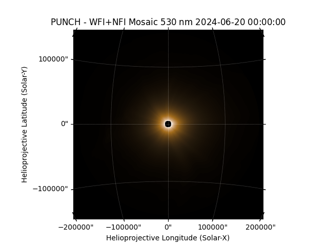
data_map.plot(norm="log")
plt.show()
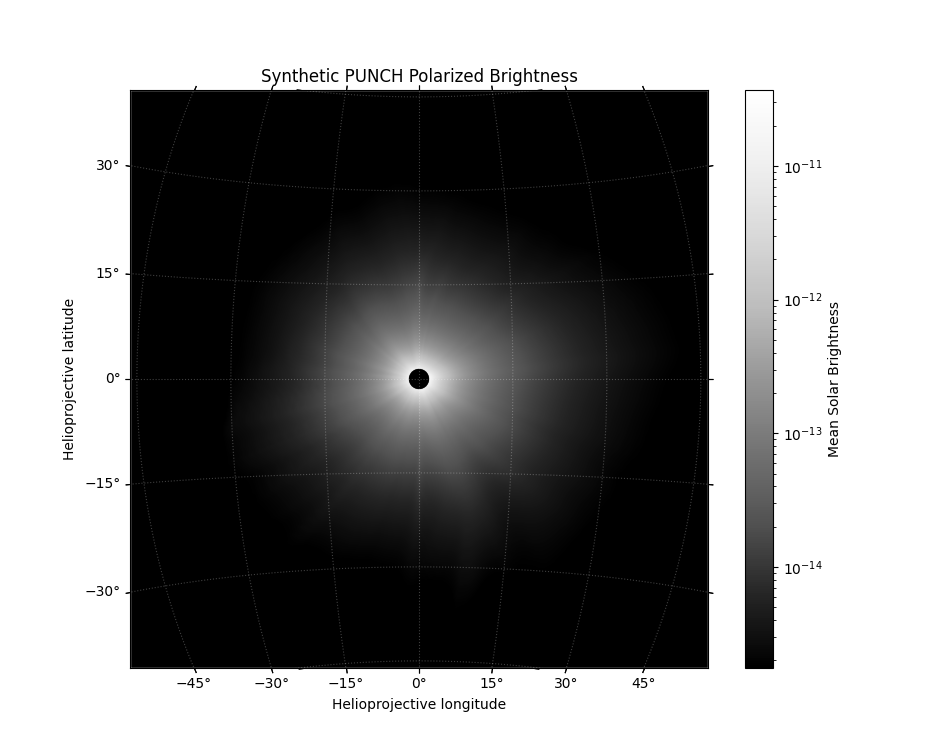
We can also use Matplotlib directly to modify the plot however we want. Notice that we set the projection so it is coordinate aware. Remember we have to slice the WCS as data_wcs[0] instead of data_wcs because our data are 3D but we want to view only the spatial dimensions.
Plot the data using matplotlib manually
fig, ax = plt.subplots(figsize=(9.5, 7.5), subplot_kw={"projection":data_wcs[0]})

im = ax.imshow(data[1], cmap="Greys_r", norm=LogNorm(vmin=1.77e-15, vmax=3.7e-11))

# set up the axis labels
lon, lat = ax.coords
lat.set_ticks(np.arange(-90, 90, 15) * u.degree)
lon.set_ticks(np.arange(-180, 180, 15) * u.degree)
lat.set_major_formatter("dd")
lon.set_major_formatter("dd")
ax.set_facecolor("black")
ax.coords.grid(color="white", alpha=.25, ls="dotted")
ax.set_xlabel("Helioprojective longitude")
ax.set_ylabel("Helioprojective latitude")
ax.set_title("Synthetic PUNCH Polarized Brightness")
fig.colorbar(im, ax=ax, label="Mean Solar Brightness")
plt.show()
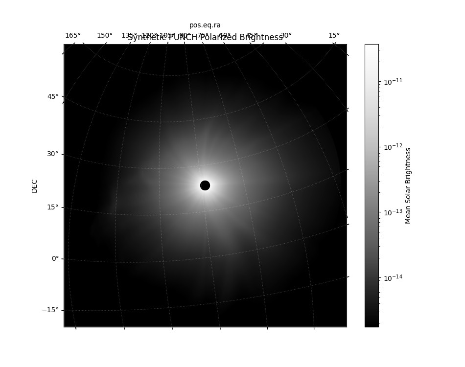
Since we set the projection, we could also use the celestial WCS instead.
Plot the data using matplotlib manually, using the celestial frame
fig, ax = plt.subplots(figsize=(9.5, 7.5), subplot_kw={"projection":data_wcs_celestial[0]})

im = ax.imshow(data[0], cmap="Greys_r", norm=LogNorm(vmin=1.77e-15, vmax=3.7e-11))

# set up the axis labels
lon, lat = ax.coords
lat.set_ticks(np.arange(-90, 90, 15) * u.degree)
lon.set_ticks(np.arange(-180, 180, 15) * u.degree)
lat.set_major_formatter("dd")
lon.set_major_formatter("dd")
ax.set_facecolor("black")
ax.coords.grid(color="white", alpha=.25, ls="dotted")
ax.set_xlabel("RA")
ax.set_ylabel("DEC")
ax.set_title("Synthetic PUNCH Polarized Brightness")
fig.colorbar(im, ax=ax, label="Mean Solar Brightness")
plt.show()
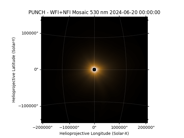
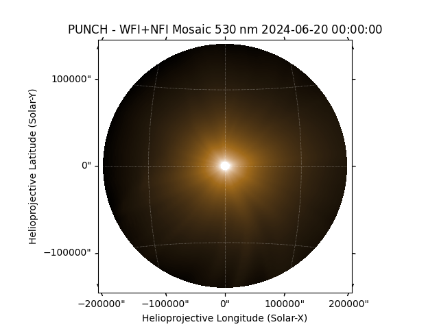
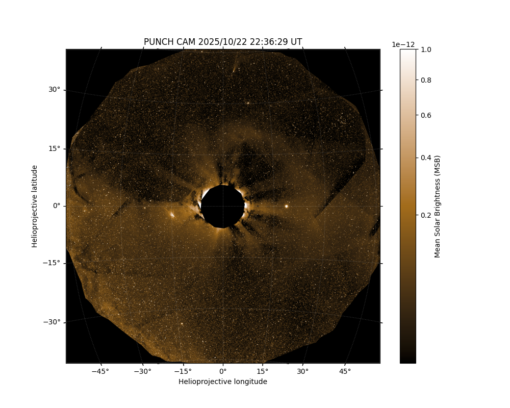
Alternatively we can use a built-in plotter function, which can be configured to plot in many of the same ways. Let try this with some real PUNCH CAM data.
Plot the data using the punchbowl plot_punch function
fig, ax = plot_punch(PUNCH_CAM)
Reprojecting the data#
What if we want want to manipulate the images? We can use built-in tools of SunPy Maps. For example, we can reproject.
What if we wanted to reproject the data to a new arbitrary coordinate frame? First, define a new target WCS
new_wcs = deepcopy(data_map.wcs)
new_wcs.wcs.ctype = "HPLN-ARC", "HPLT-ARC"
new_wcs.wcs.cunit = "deg", "deg"
new_wcs.array_shape = 1024, 1024
new_wcs.wcs.crpix = 512, 512
new_wcs.wcs.crval = 10, 10
new_wcs.wcs.cdelt = 0.0225, 0.0225
new_wcs.wcs.pc = (0.66,-0.33), (0.33,0.66)

# We can then reproject using SunPy maps
new_map = data_map.reproject_to(new_wcs)
new_map.plot()
plt.show()
Using NDCube#
So far, we’ve only talked about directly manipulating the data or using SunPy Maps. However, we encourage you to utilize NDCubes. We use them in the data reduction pipeline too. [NDCube](https://docs.sunpy.org/projects/ndcube/en/stable/introduction.html) is a SunPy package for generalized n-dimensional data. We can use our manually loaded data to make an NDCube with all of the data in one place. There’s even a way to bundle uncertainty directly into the cube.
data_ndcube = NDCube(data, wcs=data_wcs, meta=header, uncertainty=uncertainty)
print(data_ndcube)
INFO: uncertainty should have attribute uncertainty_type. [astropy.nddata.nddata]
NDCube
------
Shape: (2, 4096, 4096)
Physical Types of Axes: [('phys.polarization.stokes',), ('custom:pos.helioprojective.lon', 'custom:pos.helioprojective.lat'), ('custom:pos.helioprojective.lon', 'custom:pos.helioprojective.lat')]
Unit: None
Data Type: float32
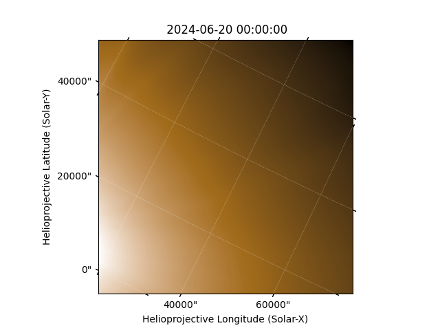
We can then use all the great NDCube functionality! Much like SunPy Maps we can reproject even. Note that as of writing this guide, the uncertainty is dropped when NDCube reprojects data.
make a target WCS
new_wcs = deepcopy(data_wcs)
new_wcs.wcs.ctype = "HPLN-ARC", "HPLT-ARC", "STOKES"
new_wcs.wcs.cunit = "deg", "deg", ""
new_wcs.array_shape = 2, 1024, 1024
new_wcs.wcs.crpix = 0, 0, 0
new_wcs.wcs.crval = 0, 0, 0
new_wcs.wcs.cdelt = 0.0225, 0.0225, 1.0

new_cube = data_ndcube.reproject_to(new_wcs)
new_cube.plot()
plt.show()
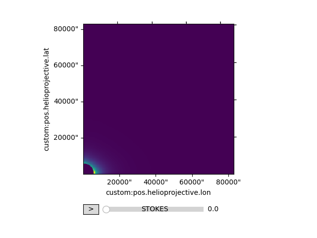
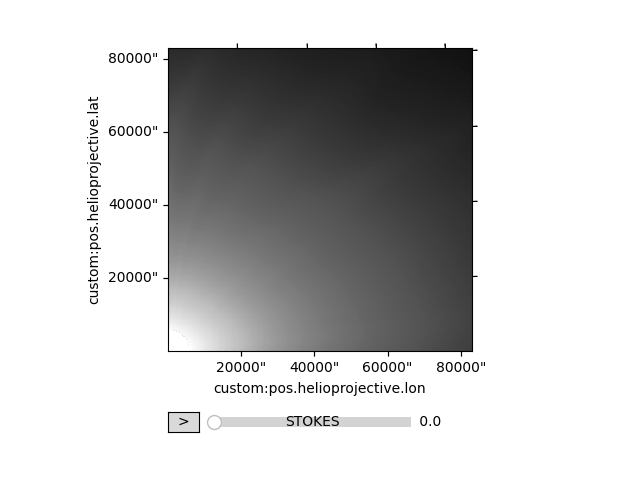
NDCubes have a plotter on them too. Notice we even get an interactive slider to manipulate the polarization axis.
new_cube.plot(interpolation="None", norm=LogNorm(vmin=1.77E-15, vmax=3.7E-11), cmap="Greys_r")
plt.show()
We encourage you to explore NDCube more. There are other helpful things like [cropping](https://docs.sunpy.org/projects/ndcube/en/stable/generated/gallery/slicing_ndcube.html#cropping-cube-using-world-coordinate-values-using-ndcube-ndcube-crop) that you can do.
Uncertainty#
Level 1, 2, and 3 PUNCH products come with an uncertainty estimate. This uncertainty is expressed as the fractional uncertainty ranging from 0 to 1. To get the absolute uncertainty, simply multiply the fractional uncertainty by the data value.
There’s an extra step though. Uncertainty is encoded as an integer in the FITS file to save space. When we inspect the uncertainty, we see it ranges from 0 to 255. Here, 255 corresponds to a fractional uncertainty of 1.0 or complete uncertainty.
print(uncertainty.min(), uncertainty.max())  # values range from 0 to 255

absolute_uncertainty = uncertainty.astype(float) / 255 * data
print(absolute_uncertainty.min(), absolute_uncertainty.max())  # now the uncertainty is in the same units as the data
1 255
0.0 3.780833285338403e-11
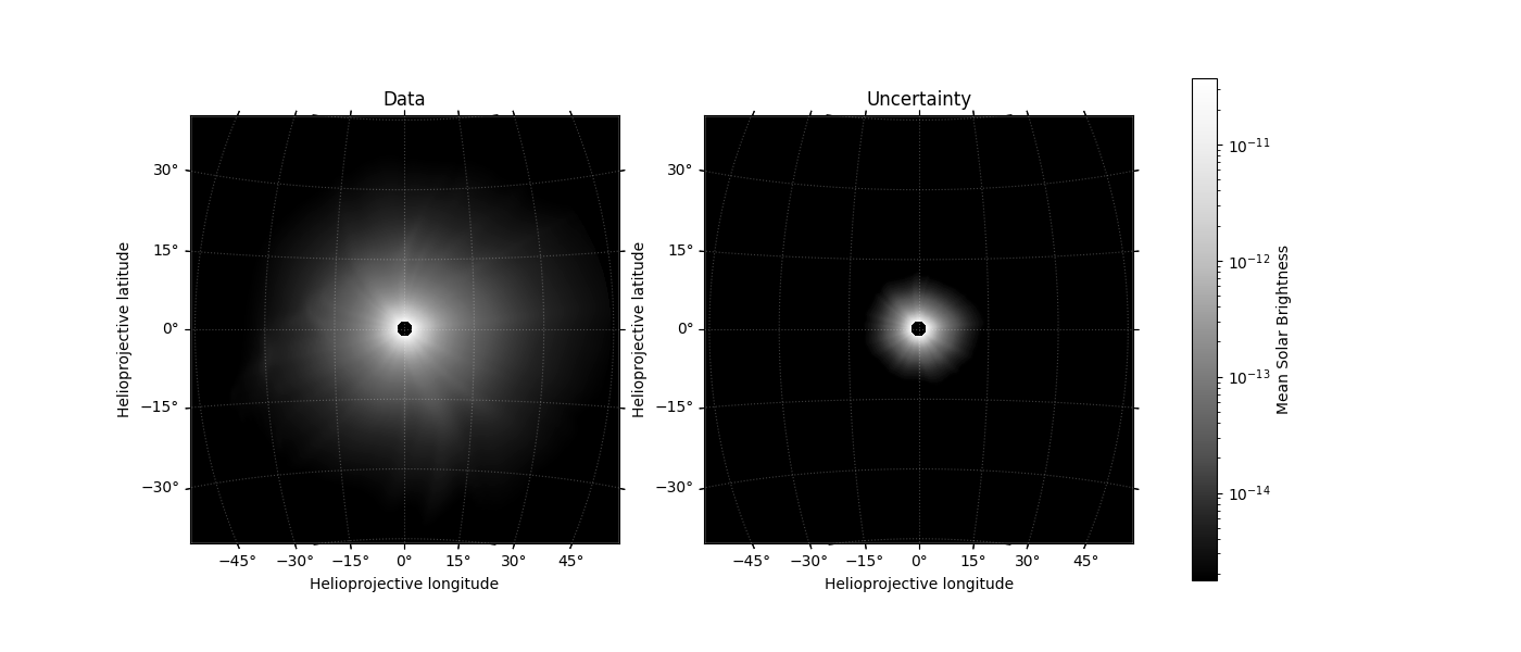
Let’s plot the data and uncertainty to get a feel for it. As mentioned earlier, analysis and visualization tools that make this easier will be released with the punchbowl package.
vmin, vmax = 1.77E-15, 3.7E-11

fig, axs = plt.subplots(figsize=(14, 6), ncols=2, subplot_kw={"projection":data_wcs[0]})

im = axs[0].imshow(data[0], norm=LogNorm(vmin=vmin, vmax=vmax), interpolation="None", cmap="Greys_r")
axs[0].set_title("Data")

axs[1].imshow(absolute_uncertainty[0], norm=LogNorm(vmin=vmin, vmax=vmax), interpolation="None", cmap="Greys_r")
axs[1].set_title("Uncertainty")

fig.colorbar(im, ax=axs, label="Mean Solar Brightness")

# set up the axis labels
for ax in axs:
    lon, lat = ax.coords
    lat.set_ticks(np.arange(-90, 90, 15) * u.degree)
    lon.set_ticks(np.arange(-180, 180, 15) * u.degree)
    lat.set_major_formatter("dd")
    lon.set_major_formatter("dd")
    ax.set_facecolor("black")
    ax.coords.grid(color="white", alpha=.25, ls="dotted")
    ax.set_xlabel("Helioprojective longitude")
    ax.set_ylabel("Helioprojective latitude")
plt.show()
Total running time of the script: (0 minutes 10.313 seconds)